Web scraping herbicide weed resistance data
 Image credit: Jo Jo
This post is originally from Open Weed Science
Web scraping
Web scraping, web harvesting, or web data extraction is data scraping used for extracting data from websites. Web pages use HyperText Markup Language (HTML). HTML isn’t a programming language like R. However, it’s a markup language with its own syntax and rules. In addition, Cascading Style Sheets, or CSS, is a language for adding styles to HTML pages.
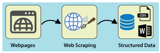
This post will lead you to get a structured data of herbicide weed resistance by country from the http://weedscience.org/Home.aspx website. We are not gonna teach you about the full details of web scraping. Rather we are using some of web scraping techniques in R to get herbicide resistance data.
If you want to learn more details about web scraping in R, please read here
Herbicide resistance
It is not novel that herbicide resistance is a major problem worldwide. If you are a student, Professor, extension or industry personnel in the field of Weed Science, you have probably landed in the The International Herbicide-Resistant Weed Database (http://weedscience.org/Home.aspx), which is leaded by Dr. Ian Heap.
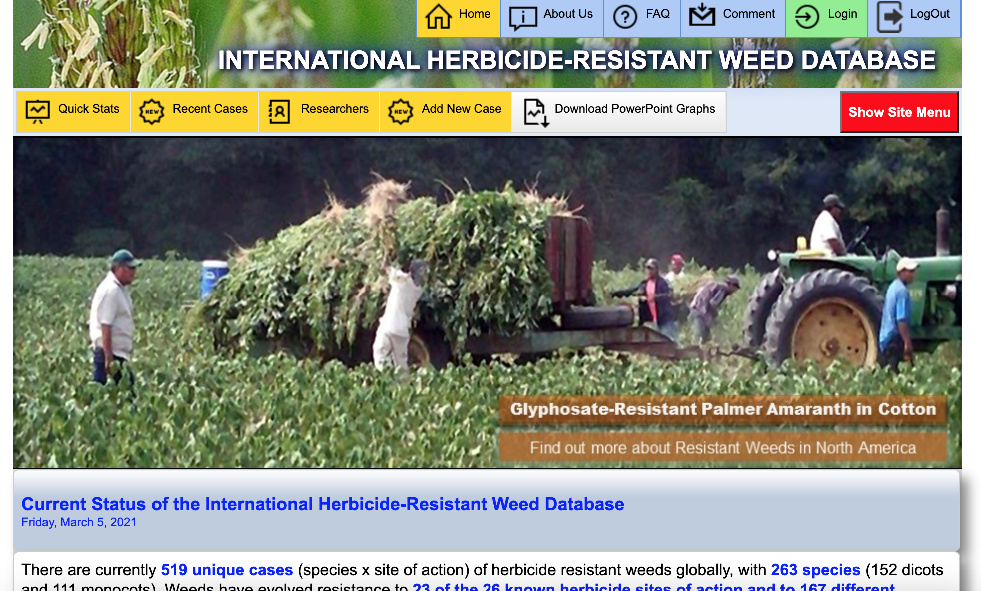
If you are a novice in Weed Science, here is the website description:
The International Survey of Herbicide Resistant Weeds is a collaborative effort between weed scientists in over 80 countries. Our main aim is to maintain scientific accuracy in the reporting of herbicide resistant weeds globally. This collaborative effort is supported by government, academic, and industry weed scientists worldwide. This project is funded by the Global Herbicide Resistance Action Committee and CropLife International.
The website is the best resource for retrieving herbicide weed resistance data. There are many ways you can get data from this herbicide resistance database. One common method is to copy and paste data from the region or weed of iquiry into a spreadsheet or a text file to summarize. However, as you know, we are vested in making your life easier when it comes to weed science data analysis. So in this post we will show you how to extract the data and direct it into R.
Packages
For this exercise the main packages used are rvest for scraping websites and tidyverse for data manipulation. Let’s start by running the codes below.
#install.packages("rvest") #Remove # if you need to install these packages
#install.packages("tidyverse")
library(rvest)
library(tidyverse)
Scraping herbicide resistance weeds by county and site of action
Once you have loaded the package in R we will start retrieving the herbicide resistance weeds by county and site of action. The data we needed can be found in the link (http://weedscience.org/Summary/CountrySummary.aspx), see below (yellow table):
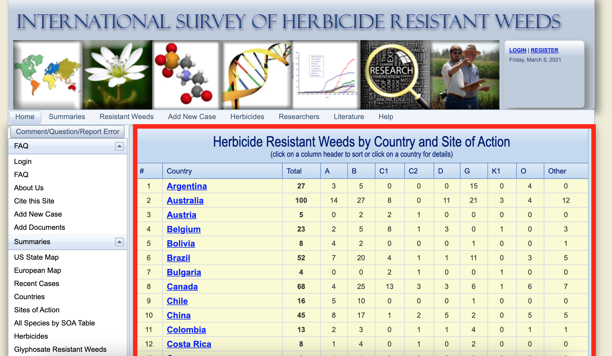
The figure above shows the web page with the data we need to retrieve. If you scroll down you can see that there are a list of 71 countries with number of herbicide resistance, total and resistance by sites of action (SOA). Notice that SOA are represented by Herbicide Resistance Action Committee (HRAC) nomenclature.
Now we need to load the web page (http://weedscience.org/Summary/CountrySummary.aspx) in R. We will use the function read_html. Let’s run the code below. Notice that “world_resistance” is the name I chose to assign the webpage information.
world_resistance <- read_html("http://weedscience.org/Summary/CountrySummary.aspx")The webpage link is now stored in “world_resistance”. We will now use two functions, html_node and html_table, to extract only the Herbicide Resistance Weeds by County and Site of Action Table. The html_node() extract the selector, which is “table” for this webpage. Then I use html_table() to make the output as a table. Notice the operator %>% is used to pass the result of one step as input for the next step.
resistance_chart <- world_resistance %>%
    html_node("table") %>% # selector = table
    html_table(fill = TRUE) # get a table

resistance_chart %>%
  slice_head(n = 5) # display 5 rows
## # A tibble: 5 x 12
## X1 X2 X3 X4 X5 X6 X7 X8 X9 X10 X11 X12
## <chr> <chr> <chr> <chr> <chr> <chr> <chr> <chr> <chr> <chr> <chr> <chr>
## 1 Herbicide R… <NA> <NA> <NA> <NA> <NA> <NA> <NA> <NA> <NA> <NA> <NA>
## 2 # Coun… Total A B C1 C2 D G K1 O Other
## 3 1 Arge… 28 3 5 0 0 0 16 0 4 0
## 4 2 Aust… 102 14 27 8 0 11 21 3 4 14
## 5 3 Aust… 5 0 2 2 1 0 0 0 0 0Notice that the output of “resistance_chart” is not tidy yet (and you know we like our data tidy, don’t we!?). We will use package janitor functions row_to_names() and clean_names() to adjust the table header.
resistance_chart1 <- resistance_chart %>%
  janitor::row_to_names(row_number = 2) %>% # make second column header
  janitor::clean_names() %>% # clean header
  as_tibble() %>% # tibble is better than data.frame
  mutate_at(vars(-country), as.integer) # make column numbers as integers
You can see that table is tidy and ready to be used as your needs (much better, yes?). If needed, an additional step is to make a single column combining all sites of action columns, here described as letters.
resistance_chart2 <- resistance_chart1 %>%
  pivot_longer(cols = a:other, # select columns to pivot
               names_to = "soa", # new column name
               values_to = "resistant") # new values column name

resistance_chart2
## # A tibble: 639 x 5
## number country total soa resistant
## <int> <chr> <int> <chr> <int>
## 1 1 Argentina 28 a 3
## 2 1 Argentina 28 b 5
## 3 1 Argentina 28 c1 0
## 4 1 Argentina 28 c2 0
## 5 1 Argentina 28 d 0
## 6 1 Argentina 28 g 16
## 7 1 Argentina 28 k1 0
## 8 1 Argentina 28 o 4
## 9 1 Argentina 28 other 0
## 10 2 Australia 102 a 14
## # … with 629 more rowsScraping herbicide resistant weeds with detail information
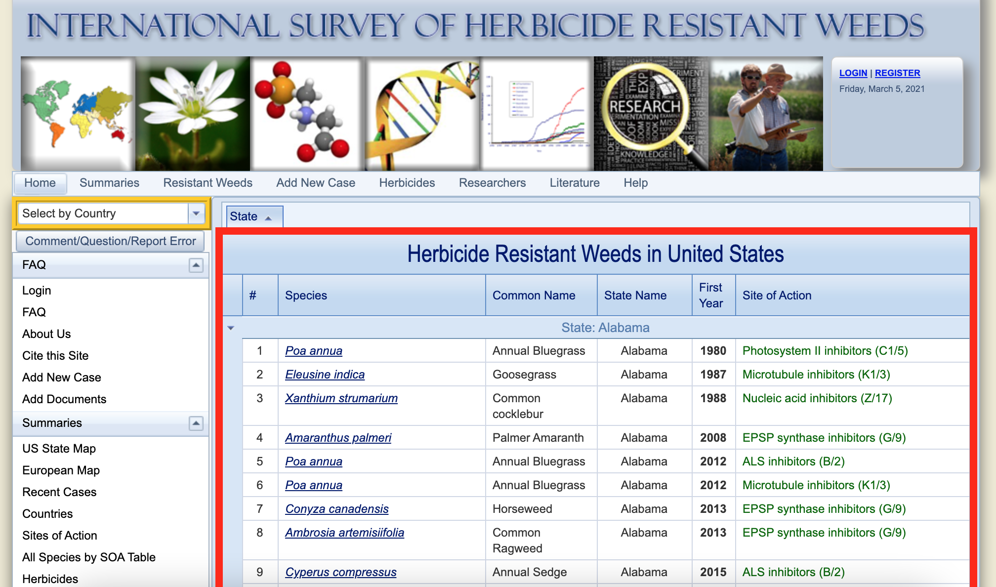
You might be interested in selecting herbicide resistant weeds data in a country of your choice. Here we will show how to extract herbicide resistance data from all 71 countries listed in the Heap et al. (2021) database. The gif below demonstrates the data that we are retrieving from the website.
I clicked on United States to show the data that we are retrieving from the website but we will get that data from all 71 countries listed.
The link below show an example of the data we are are interested. Notice the website link changed a bit when we click on United States: http://weedscience.org/Summary/Country.aspx?CountryID=45. If you look closely, the only thing is changing is the last attribute of the link, ID. Each country has their own code ID. The United States ID is 45.
Knowing that we can extract all 71 countries’ data at once. We will use a similar code snippet, as demonstrated earlier in this post. The difference is that we are using the codes inside a function (country_function) that takes the country id as an argument and pass into the function body.
country_function <- function(id) {

  url <- paste0("http://weedscience.org/Summary/Country.aspx?CountryID=",id,"")
  #id will change by each country id number

  # Read url
  resistance <- read_html(url)

  # Extract herbicide resistance data
  chart <- resistance %>%
    html_node(".rgMasterTable") %>% # selector
    html_table(fill = TRUE) # get the table

  # Tidy dataset
  final_chart <- chart %>%
    janitor::row_to_names(row_number = 2) %>% # make second column header
    janitor::clean_names() %>% # clean header
    as_tibble() %>% # tibble is better than data.frame
    drop_na() %>% # drop NA values
    mutate_at(c("number", "first_year",
                "country_id", "resist_id"),
              as.integer) # make columns numbers as integer
  # Get final dataset
  final_chart
}
Now, the function is done and we want to test it. Lets use id = 1 to see the output.
country_function(id = 1)## # A tibble: 153 x 10
## x number species common_name country state_name first_year country_id
## <chr> <int> <chr> <chr> <chr> <chr> <int> <int>
## 1 "" 1 Lolium r… Rigid Ryegra… Austra… New South… 1985 1
## 2 "" 2 Avena st… Sterile Oat Austra… New South… 1989 1
## 3 "" 3 Avena fa… Wild Oat Austra… New South… 1991 1
## 4 "" 4 Cyperus … Smallflower … Austra… New South… 1994 1
## 5 "" 5 Sagittar… California A… Austra… New South… 1994 1
## 6 "" 6 Damasoni… Starfruit Austra… New South… 1994 1
## 7 "" 7 Sisymbri… Oriental Mus… Austra… New South… 1994 1
## 8 "" 8 Sinapis … Wild Mustard Austra… New South… 1996 1
## 9 "" 9 Phalaris… Hood Canaryg… Austra… New South… 1997 1
## 10 "" 10 Lolium r… Rigid Ryegra… Austra… New South… 1997 1
## # … with 143 more rows, and 2 more variables: site_of_action <chr>,
## # resist_id <int>Great! The function works.

It gets the data from Australia, which means that the Australia ID in this website is 1. However, countries are listed alphabetically here: http://weedscience.org/Summary/CountrySummary.aspx. Therefore, I was expecting Argentina to be id = 1, not Australia.
It turns out that id number is not following the alphabetical order.

Fear not, we’ve got a plan.
After some workarounds I have gotten the full country name and id number.
country <- tribble(
~country_name, ~id,
"argentina", 48,
"australia", 1,
"austria", 2,
"belgium ", 3,
"bolivia", 4,
"brazil", 5,
"bulgaria", 6,
"canada", 7,
"chile", 8,
"china", 9,
"colombia", 10,
"costa rica", 11,
"czech republic", 12,
"denmark", 13,
"ecuador", 14,
"egypt", 15,
"fiji", 16,
"france", 17,
"germany", 18,
"greece", 19,
"hungary", 20,
"india", 21,
"indonesia", 22,
"israel", 23,
"italy", 24,
"japan", 25,
"kenya", 26,
"south korea", 27,
"malaysia", 28,
"mexico", 29,
"new zealand", 30,
"norway", 31,
"philippines", 32,
"poland", 33,
"portugal", 34,
"saudi arabia", 35,
"slovenia", 36,
"south africa", 37,
"spain", 38,
"sri lanka", 39,
"sweden", 40,
"switzerland", 41,
"taiwan", 42,
"netherlands", 43,
"united kingdom", 44,
"united states", 45,
"paraguay", 46,
"thailand", 47,
"cyprus", 53,
"jordan", 55,
"nicaragua", 60,
"russia", 65,
"syria", 69,
"turkey", 71,
"uruguay", 73,
"ethiopia", 76,
"tunisia", 78,
"iran", 79,
"venezuela", 80,
"ireland", 81,
"panama", 82,
"el salvador", 83,
"guatemala", 84,
"honduras", 85,
"pakistan", 86,
"finland", 139,
"kazakhstan", 157,
"latvia", 174,
"lithuania", 185,
"serbia", 245,
"ukraine", 230
)

country
## # A tibble: 71 x 2
## country_name id
## <chr> <dbl>
## 1 "argentina" 48
## 2 "australia" 1
## 3 "austria" 2
## 4 "belgium " 3
## 5 "bolivia" 4
## 6 "brazil" 5
## 7 "bulgaria" 6
## 8 "canada" 7
## 9 "chile" 8
## 10 "china" 9
## # … with 61 more rowsOnce you have the data set with country and id number, we can iterate with map function from purrr package.
resistance_data <- country %>%
  arrange(country_name) %>% #arrange country in alphabetical order
  mutate(resistance_data = map(id, country_function)) # iterate function over id

# resistance data is in a list by each country
resistance_data
## # A tibble: 71 x 3
## country_name id resistance_data
## <chr> <dbl> <list>
## 1 "argentina" 48 <tibble [29 × 9]>
## 2 "australia" 1 <tibble [153 × 10]>
## 3 "austria" 2 <tibble [4 × 9]>
## 4 "belgium " 3 <tibble [21 × 9]>
## 5 "bolivia" 4 <tibble [8 × 9]>
## 6 "brazil" 5 <tibble [54 × 9]>
## 7 "bulgaria" 6 <tibble [4 × 9]>
## 8 "canada" 7 <tibble [118 × 10]>
## 9 "chile" 8 <tibble [19 × 9]>
## 10 "china" 9 <tibble [44 × 9]>
## # … with 61 more rowsFinally, we use unnest function to unlist the resistance_data.
final_resistance_data <- resistance_data %>%
  unnest(resistance_data) %>% # unlist resistance data
  dplyr::select(-x) # removing column x
Final herbicide weed resistance data
The “final_resistance_data” contains the full resistance dataset of all 71 countries listed in Heap et al. (2021). There are many possibilities when working with this data. For example, you can filter it by your country, weeds and/or use visualization. Its up to you!
We would like to thank Heap at al. (2021) for providing this great herbicide resistance database and all of the weed scientist collaborators that submit data for reporting.
Citation
Heap, I. The International Survey of Herbicide Resistant Weeds. Online. Internet. Friday, March 5, 2021.