2020 WSSA/WSWS Meeting Program Text Analysis

Last updated on Oct 15, 2020 11 min read

Image credit: Max Chen

This post is also published on the Open Weed Science website.

Conference

The 2020 Weed Science Society of America (WSSA) and Western Society of Weed Science (WSWS) joint meeting will be held on Mar 2-5 in Maui (http://wssa.net/meeting/2020-annual-meeting/), Hawaii. Unfortunately, some of us will not be present at the meeting but the data analysis discussed herein can help you learn the main Weed Science topics to be discussed in Hawaii.

Analysis

The goal of this text analysis is to evaluate the frequency of words in the 2020 WSSA/WSWS oral and poster titles. The 2020 WSSA program is available as a pdf file. In order to achieve our goal with this exercise, you have to download the pdf, load it in R, organize the selected words in a data frame, then in a corpus (collection of text document). Every text analysis requires creating a corpus. In this case, each text document in corpus must be a word. You will see that the process from pdf to corpus requires creating and binding data frames, using loop functions and other tools specific for text mining in R. Finally, we use ggplot and wordcloud to display the results.

If you want to learn how to analyze the WSSA/WSWS program, we encourage you to read this post in detail.

If you are not interested in learning the analysis itself, scroll down to Results.

Install packages

The text analysis of the WSSA/WSWS program will be performed in R statistical software. In order to accomplish this exercise, you will need to install the following R packages:

install.packages(downloader)
install.packages(tidyverse)
install.packages(pdftools)
install.packages(wordcloud)
install.packages(topicmodels)
install.packages(tm)
install.packages(rcorpora)

Run the codes above by clicking in the “Run” option on the top right corner of you R script or R markdown. These codes will install the necessary packages for text analysis. Once you install these packages you will not need to install them again, unless you update R and/or RStudio.

Import the text

First you need to find the conference program, which is available in the WSSA website (http://wssa.net/meeting/2020-annual-meeting/):

Figure

You can either save the pdf program in your local folder together with your R files, or you could use R to download the pdf:

library(downloader)

Copy and past the pdf link to the function download, notice that I named the pdf as ‘wssa.pdf’. The pdf will be saved in your local folder.

download function

wssa <- download("http://wssa.net/wp-content/uploads/2020-Program_1_29_Final.pdf", "wssa.pdf", mode = "wb")

Load the pdf file

Now, you need to load the pdf in R with pdf_text function. The pdf_text loads the pdf in R and strsplit function breaks the lines in pdf pages.

library(tidyverse)

pdf_text function

strsplit function

pdf_full <- pdf_text("wssa.pdf") %>% 
  strsplit(split = "\n")

Text analysis

The WSSA/WSWS program (pdf file) contains 155 pages. My goal is to select only the title words of poster and oral presentations.

Select pages needed

We have selected pages 15 to 114 because we are only interested in title words.

title <- pdf_full[15:114]

For the text analysis, we need to create a single word vector. The title contains the selected WSSA program pages needed to reach our goal but it is a list of vectors not a single vector.

Loop

As described above, nearly 100 pages were selected from the WSSA/WSWS annual meeting program. First, we need to organize the text (title) in a data frame. It would take a long time to convert the list of vectors into a single vector, and then a data frame. Therefore, a loop function is used herein to expedite the process:

titledm <- data.frame() # as data frame
for (i in 1:length(title)) {
  print(i)
  titlelines <- data.frame(names = title[[i]])
  titledm <- bind_rows(titledm, titlelines)
}

The loop function created a data frame with a single variable (names), which is a character vector.

head(titledm, n=5)

##                                        names
## 1                                    PROGRAM
## 2                   MONDAY AFTERNOON MARCH 2
## 3                            General Session
## 4       LOCATION:              Monarchy #1-4
## 5 TIME:                  04:00 PM - 06:00 PM

As you can see, there are more than a word in each row.

Tokens for titles

Tokenization is the act of breaking up a sequence of strings into pieces such as words, keywords, phrases, symbols and other elements called tokens.

library(tidytext)

Befere tokenization, there is onr issue, a common and important name for our analysis is the herbicide 2,4-D. If we do tokenization with 2,4-D, the function will break thw word in 2, 4, -, and D; thus the word will disappear. Changing how 2,4-D is written is a solution to keep it in the analysis.

titledm$names <- gsub("2,4-D" , "twofourd" , titledm$names)

Now that 2,4-D is named twofourd, we can proceed with tokenization.

unnest_tokens function

title_tokens <- titledm %>%
  unnest_tokens(words, names)

Let’s run title_tokens to see how the data are organized. Please notice that each row contains a word or number.

head(title_tokens, n=5)

##         words
## 1     program
## 2      monday
## 2.1 afternoon
## 2.2     march
## 2.3         2

Removing authors’ name

There are authors’ names and addresses below the titles in the selected pages. It is not our goal to analyze authors’ names; therefore, we have to remove authors’ name from the selected pages. The author index of WSSA/WSWS program is available in pages 116 to 146. Similarly to titles, I will select those pages, do a another loop and create a vector of authors’ names.

authors <- pdf_full[116:146]
authorsdm <- data.frame()
for (i in 1:length(authors)) {
  print(i)
  authorslines <- data.frame(names = authors[[i]])
  authorsdm <- bind_rows(authorsdm, authorslines)
} 
#tokerization
authors_tokens <- authorsdm %>%
  unnest_tokens(words, names)

So far, there are two important vectors, a vector of words from page 15 to 114 (title_tokens) and a vector from page 116 to 146 (authors_tokens). To achieve our goal of removing authors’ name from title pages (title_tokens), a simple solution is to use the anti_join funtion, which removes all words (first and last authors’ names) presented in authors_tokens from title_tokens.

anti_join funtion

titles_tokens_clean <- anti_join(title_tokens, authors_tokens, by = "words")

New created vector

A new vector is named titles_tokens_clean.

head(titles_tokens_clean, n = 6)

##         words
## 1     program
## 2.1 afternoon
## 2.2     march
## 3     general
## 3.1   session
## 4    location

A issue that we found is some authors have a number after their last names below the titles. For example Lindquist1, Yearka2, Tenhumberg1, Jhala1, and Werle3, numbers are given to identify their respective institutions.

Figure

A solution for this problem is to create a data frame with authors’s last names with numbers from 1 to 12. To accomplish this task, we need the loop function again. This is the third loop in this text analysis; by the end of this exercise you will become an expert in using the loop function :)

rm_author <- c(1:12) 
rm_authors_number <-c()
for (i in 1:length(rm_author)) {
  print(i)
  rm_authors_numbers <- c(paste0(authors_tokens$words, i))
  rm_authors_number <- c(rm_authors_number, rm_authors_numbers)
}

Now, let’s create a data frame with column as character.

rm_authors <- data.frame(rm_authors_number) 
rm_authors <- rename(rm_authors, words = rm_authors_number) 
rm_authors$words <- as.character(rm_authors$words)

rm_authors <- data.frame(rm_authors_number) 
rm_authors <- rename(rm_authors, words = rm_authors_number) 
rm_authors$words <- as.character(rm_authors$words)

Similarly, we run the anti_join funtion again to remove the last names with numbers for our main data frame, now named titles_clean_clean.

titles_clean_clean <- anti_join(titles_tokens_clean, rm_authors, by = "words")

head(titles_clean_clean, n=10)

##         words
## 1     program
## 2.1 afternoon
## 2.2     march
## 3     general
## 3.1   session
## 4    location
## 4.1  monarchy
## 5        time
## 5.1        04
## 5.2        00

Stop words

There are some words that we are not interested in, such as march, afternoon, numbers (04, 00), penn etc. Thus, we need to clean the vector titles_tokens_clean.

Stop words are words we may want to remove from the text analysis. For example, we used the package rcorpora to remove words of geography (country, city, capitals, state) and English words such as “a”, “and”, “the”, “of”, “as” etc.

library(rcorpora)

# cities and states
geography <- corpora("geography/us_cities") 
cities <- geography$cities
stopwords_cities <- c(cities$city) # stop cities words 
stopwords_cities <- tolower(stopwords_cities)  # making small caps
stopwords_state <- c(cities$state) # stop state words 
stopwords_state <- tolower(stopwords_state) # making lowercase
#country
country <- corpora("geography/countries") # stop country words 
stopwords_countries <- c(country$countries) # stop countries words 
stopwords_countries <- tolower(stopwords_countries) # making lowercase
#capitals
capitals <- corpora("geography/us_state_capitals")
capitals <- c(capitals$capitals)  # stop US capital words 
stopwords_capitals <- c(capitals$capital) # stop us capitals words 
stopwords_capitals <- tolower(stopwords_capitals) # making lowercase
#english
Enlish <-corpora("words/stopwords/en")  
stopwords_en <- c(Enlish$stopWords) # stop english words 
stopwords_en <- tolower(stopwords_en) # making lowercase

The codes above created vectors of capitals, cities, states, country, and English words. Sometimes, the stop words may not be enough, which is the case for the WSSA/WSWS analysis. In this case, we had to manually create a vector of stop words.

# words that we want to avoid in the text analysis
stop_wssaprogram_words <- c("university", "universidad", "universidade", "location",    
                      "agriscience", "usda", "monarchy", "north", "march", "moderator",
                      "extension", "college", "tech", "time", "student", "contest",
                      "break", "station", "basf", "division", "ars", "fort", "guelph",
                      "presenter", "maui", "monday", "tuesday", "wednesday", "thursday",
                      "oral", "poster", "united", "western", "speaker", "science", "lleida",
                      "dakota", "agriculture", "service", "laramie", "forest", "piracicaba",
                      "purdue", "agrilife", "center", "syngenta", "morning", "afternoon",
                      "agri", "ventenata", "center", "east", "food", "tifton", "adelaide",
                      "pullman", "resources", "affiliation", "saskatoon", "saskatchewan",   
                      "moscow", "park", "suite", "west", "corteva", "bayer", "frankfurt",
                      "cropscience", "beltsville", "south", "northeast", "northern",  
                      "northwest", "platte", "central", "cooperative", "cornell", "phd",
                      "program", "maui", "clemson", "stoneville", "baton", "rouge",
                      "ridgetown", "buenos", "ithaca", "são", "cordoba", "usa", "carbondale",
                      "sur", "river", "system", "johnson", "athens", "city", "usp", "paulo",
                      "pelotas", "aires", "winfield", "llc", "são", "kingdom", "pnw",
                      "lexington", "eastern", "mornings", "brookings", "southern", "federal",
                      "scottsbluff", "ontario", "manitoba", "thorntown", "lexiton",
                      "newport", "macomb", "penn", "institute", "islands", "summit",
                      "winnipeg", "saint", "fmc", "brookston", "southeastern",
                   "council", "corporation", "rio", "grande", "harrow", "aac", "aafc",
                   "beach", "aberdeen", "brunswick", "napa", "rutgers", "mills",
                   "valent","society", "starkville", "department", "sheridan", "viçosa",
                   "lonoke", "osmond", "las", "cruces", "makawao", "painter", "lethbridge",
                   "daejeon", "moghu", "bridgestone", "princeton", "lafayette", "hastings",
                   "symposium", "volcano", "colfax", "greeley", "boulder", "seffner", "des",
                   "moines", "amvac", "lees", "crawley", "kyoto", "manoa", "bonham",
                   "langley", "waipahu", "salinas", "pontotoc", "richelieu", "galena",
                   "beebe", "calgary", "bogor", "jean", "hampshire", "trinity", "triangle",
                   "york", "monticello", "bogotá", "calgary", "albion", "alegre", "arabia",
                   "saudi", "balm", "bay", "brooks", "bury", "committee", "csic", "daniel",
                   "dow", "edmonton", "edmunds", "edwardsville", "eloy", "esalq","goldsboro",
                   "hettinger", "iaa", "korea", "lacombe", "jaboticabal", "keenesburg",
                   "marina", "mcminnville", "maringa", "marrone", "morrisville", "monterey",
                   "nufarm", "oak", "ncsu", "nacional", "ottawa", "pendleton", "pat",
                   "porto", "plc", "stephenville", "steckel", "tokyo", "universitat", "vero",
                   "univ", "wageningen", "wooster", "christi", "corpus", "company", "dryden",
                   "glenn", "nice", "nrcs", "oroville", "susanville", "amworth", "yuba",
                   "hays", "bracknell", "agcenter", "americas", "america", "immokalee",
                   "harpenden", "rothamsted", "wagga", "county", "hawaiian",
                   "national", "pacific", "adams")

Now, we will combine all stop words into a single vector:

stopwords_titles <- c(stopwords_cities, stopwords_state, stopwords_countries, stopwords_capitals,
                      stopwords_en,  stop_wssaprogram_words)

Corpus

Text analysis methodology requires to convert any text being analyzed into a corpus.

library(topicmodels)
library(tm)

title_source <- VectorSource(titles_clean_clean$words)
title_corpus <- VCorpus(title_source)

Cleaning the text

Now, it is time to use all stop words (stopwords_titles) to clean the data frame.

# this code section will take long (~3 min) to run. 
clean_corpus <- function(corpus){
  corpus <- tm_map(corpus, removePunctuation) # remove punctuation
  corpus <- tm_map(corpus, content_transformer(tolower)) # remove punctuation
  corpus <- tm_map(corpus, removeNumbers) # remove numbers
  corpus <- tm_map(corpus, removeWords, stopwords_titles) # remove stop words
  corpus
}
title_corpus <- clean_corpus(title_corpus)

Creating a matrix

To plot the text analysis using wordcloud or ggplot function in R, we have to convert VCorpus format into a TermDocumentMatrix, then a data.frame.

title_dtm <- TermDocumentMatrix(title_corpus)
title_matrix <- as.matrix(title_dtm)
title_v <- sort(rowSums(title_matrix), decreasing=TRUE)
title_dt <- data.frame(word = names(title_v),freq=title_v)

Remember when we changed the 2,4-D name format? Now it is time to bring back the name 2,4-D back to the analysis.

title_dt$word <- gsub("twofourd" , "2,4-D" , title_dt$word)

We are now done with text analysis!

Results

Bar chart

The most frequent word in the the 2020 WSSA/WSWS meeting is weed (n=137). Also, the plural weeds (n=38) is shown in the WSSA/WSWS program (Figure 1).

No surprises!

title_dt %>% 
  filter(freq >= 30) %>% 
  ggplot(aes(x=reorder(word,freq), y=freq, fill=freq)) +
  scale_fill_continuous(low = "#FFF6F6", high = "#9b0000") +
  geom_col(show.legend=FALSE) + coord_flip() + theme_classic() +
  labs(y="Frequence (n)", x="Words") + ylim(0,150) +
  theme(axis.title = element_text(size=15),
        axis.text = element_text(size=13))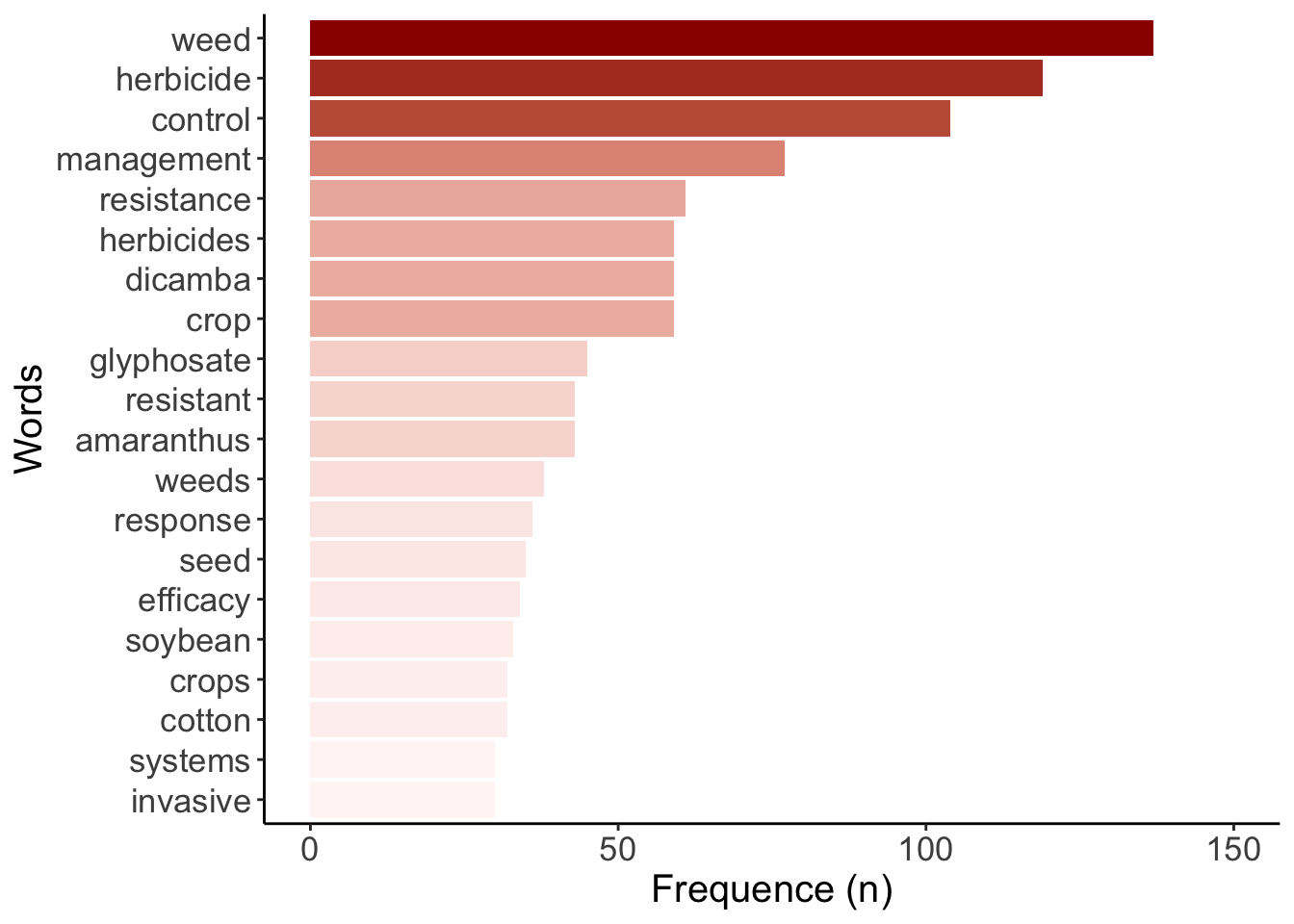

Figure 1: Most frequent words (n=30+) that appeared in the WSSA/WSWS oral and poster presentation titles.

Other words appear 30+ times in this WSSA/WSWS program:

Interesting to see how herbicide (n=119) and herbicides (n=59) used for weed control (n=104) dominate the program.
Efficacy (n=34) is also a commonly used word likely related to chemical weed management (n=77).
Dicamba (n=59) appeared more than glyphosate (n=45), likely due to recent introduction of dicamba resistant crops, benefits and some of the challenges associated with the herbicide.
In 2020, resistance (n=61), resistant (n=43), and amaranthus (n=43) are still major topics in the WSSA/WSWS meeting.
Seed (n=35) is likely due to increase research on Harrington Seed Destructor strategy for weed management.
Soybean (n=33) and cotton (n=32) are the most frequent crops mentioned in the WSSA/WSWS program.

Word cloud

The word cloud provides a big picture of the WSSA/WSWS meeting program. It shows words that appeared at least twice in the program. Bigger words indicate higher frequency in the program and vice versa. Same colors indicate word frequency of the same magnitude.

library(wordcloud)

wordcloud function

pal <- brewer.pal(8,"Dark2") #selecting the color palette
set.seed(1234)
wordcloud(words = title_dt$word, freq = title_dt$freq, min.freq=2, scale=c(5,.1),
           random.order=FALSE, rot.per=0.35, colors=pal)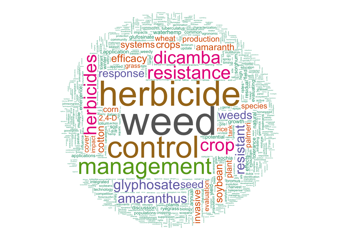

The word cloud highlights how herbicides dominate the weed science discipline.

Challenge:

What are the dominant weeds in the word cloud?
What are the dominat herbicides in the word cloud?
Can you find the words: ecosystem, ecology, sustainable and agroecosystem?

Spend some time cruising through the big and small words. What are your thoughts? Which words do you think are missing in the program? Should some words be bigger than others?

Acknowledgements

We would like to acknowledge Nick Arneson for reviewing this post

herbicide word cloud